


Density
Defines a 3D decimal value field.
Density
Constant
Outputs a constant value.
Expected Inputs: 0
Parameters:
| Name | Description |
|---|---|
| Value | Decimal number. |
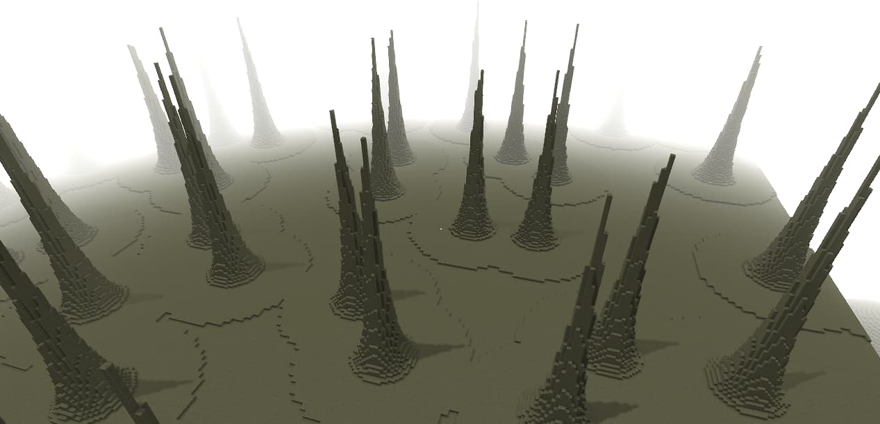
SimplexNoise2D
Outputs a value in the range [-1, 1] from a 2D Simplex noise field that varies on the x/z plane. For more details on how simplex noise works and what every parameter does to the output you can visit this page.
This node automatically caches the value per x/z column.
Expected Inputs: 0
Parameters:
| Name | Description |
|---|---|
| Lacunarity | positive decimal number. Impacts the scale of each consecutive octave. A good starting value would be 2.0, which results in each consecutive octave having details that are 2x smaller than the previous. Higher values result in grainier noise. |
| Persistence | positive decimal number. Multiplies the intensity of each consecutive octave. A good starting value would be 0.5, which results in each consecutive octave being half as strong as the previous. |
| Scale | positive decimal number. Represents the field’s period distance in blocks. Greater values stretch the noise field outward. A good starting value would be 50. |
| Octaves | integer greater than 0. Greater values result in more detail. A good starting value would be 4. Requiring values over 10 are uncommon. |
| Seed | string |
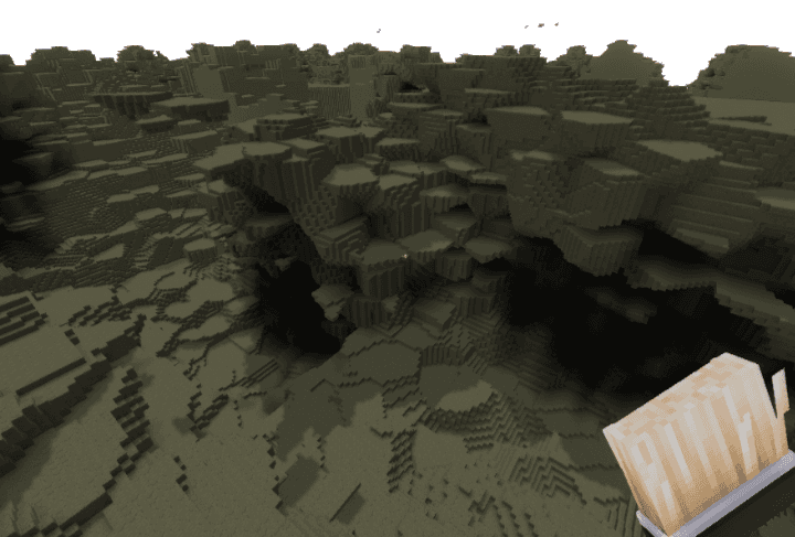
SimplexNoise3D
Outputs a value in the range [-1, 1] from a 3D Simplex noise field that varies on the x/y/z space. For more details on how simplex noise works and what every parameter does to the output you can visit this page.
Expected Inputs: 0
Parameters:
| Name | Description |
|---|---|
| Lacunarity | positive decimal number. Impacts the scale of each consecutive octave. A good starting value would be 2.0, which results in each consecutive octave having details that are 2x smaller than the previous. Higher values result in grainier noise. |
| Persistence | positive decimal number. Multiplies the intensity of each consecutive octave. A good starting value would be 0.5, which results in each consecutive octave being half as strong as the previous. |
| ScaleXZ | positive decimal number. Represents the field’s period distance in blocks on the horizontal XZ plane. Greater values stretch the noise field outward. A good starting value would be 50. |
| ScaleY | positive decimal number. Represents the field’s period distance in blocks on the vertical Y axis. Greater values stretch the noise field outward. A good starting value would be 50. |
| Octaves | integer greater than 0. Greater values result in more detail. A good starting value would be 4. Requiring values over 10 are uncommon. |
| Seed | string |
WhiteNoise
Outputs white noise in the range [-1, 1].
Expected Inputs: 0
Parameters:
| Name | Description |
|---|---|
| Seed | string |
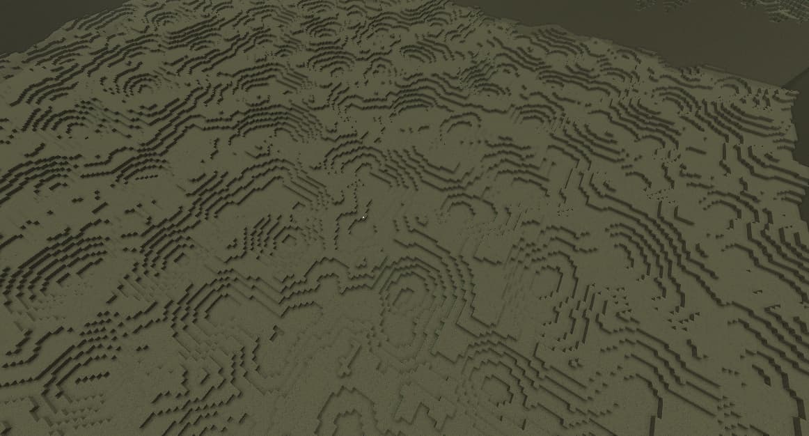
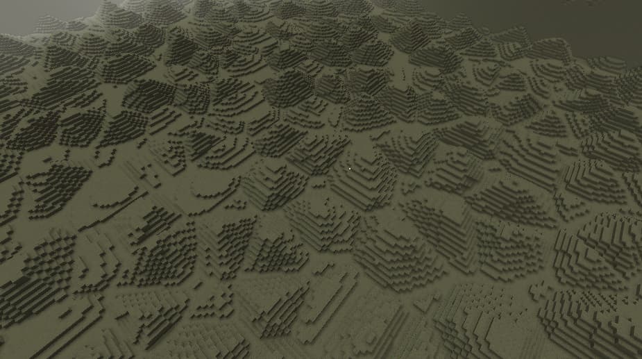
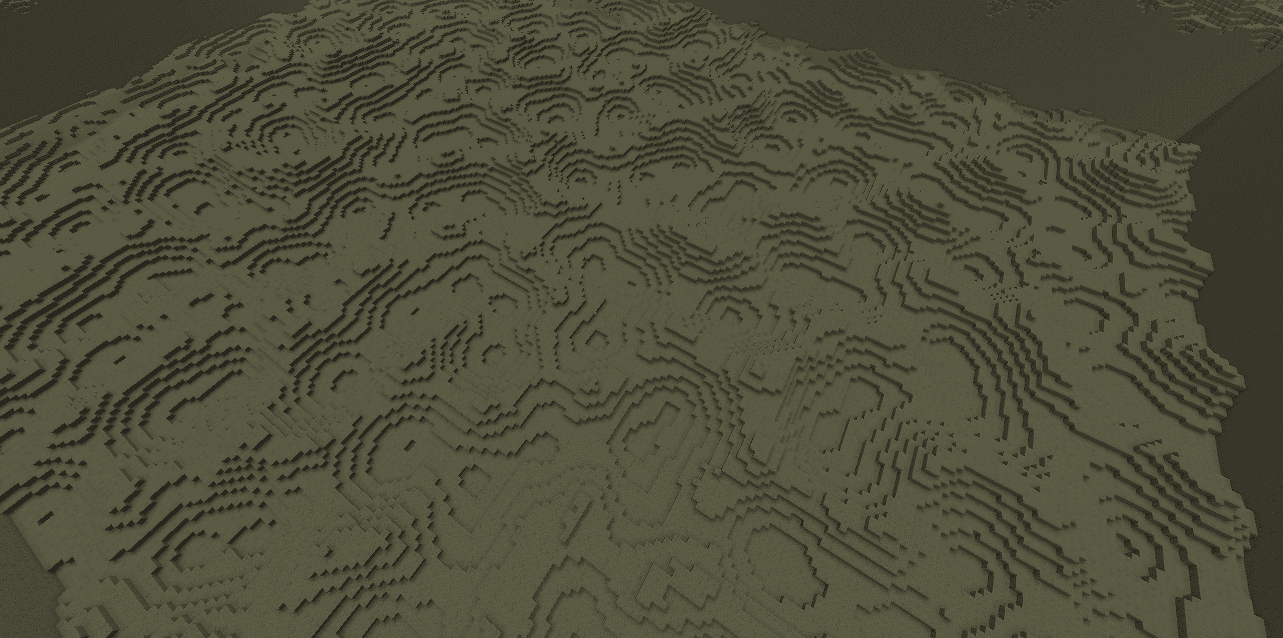
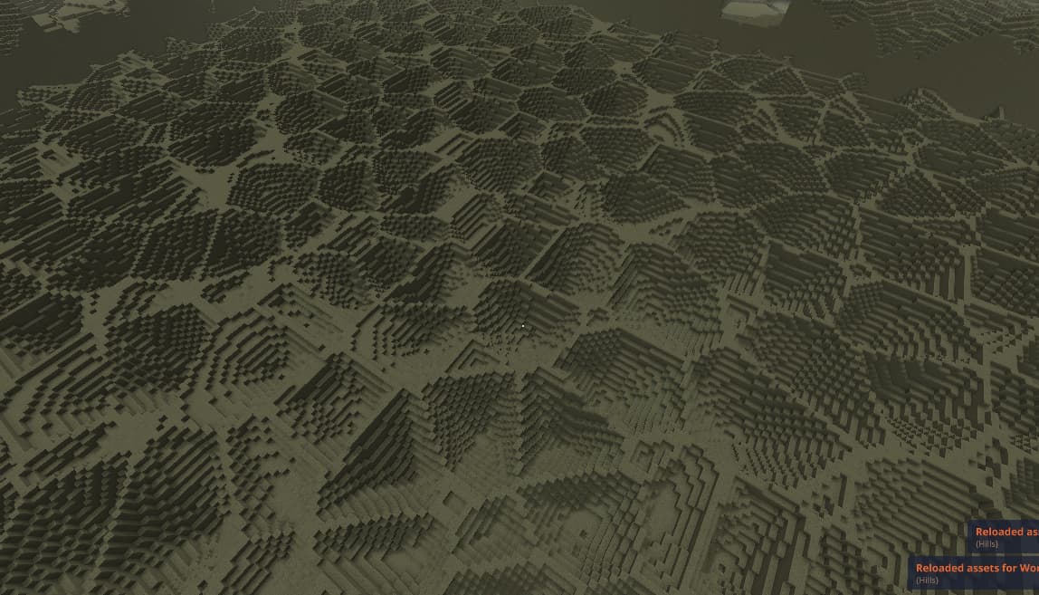
PositionsCellNoise
Produces a 2D/3D density field in which the value is determined by each coordinate’s distance from a field of Positions. You can use this asset to generate advanced Cell noise with control over the exact placement of the Cell’s through the Positions asset. You can also configure how the distance is interpreted to produce the output. You can use the traditional Cell noise ReturnTypes or create your own curves. You can also sample the Cell value from another Density field asset.

Parameters:
| Name | Description |
|---|---|
| Positions | Positions slot. This provides the Positions of each cell’s core. |
| ReturnType | ReturnType slot. This determines how the distance from each Position point is interpreted to produce the density field. |
| DistanceFunction | DistanceFunction slot. This determines how the distance is calculated. |
| MaxDistance | decimal value. The maximum distance around each Position that it has an effect on the Density field. A good starting value is putting it a bit over half the distance between two of your Position points. Greater values have a greater impact on performance. |
ReturnType
Determines how each Position point affects the Densty field around it, or how the Cell looks.
Below are the different types you can use.
CellValue
The Density value is constant inside each cell and is sampled from the provided Densty field.
The images below show a 2D and a 3D output of the CellValue return type.
Parameters:
| Name | Description |
|---|---|
| Density | Density asset slot. The Density value of each cell is sampled from this field at the cell's core Position point. |
| DefaultValue | Floating point number. This value is used outside of cells. This can happen when the field's MaxDistance value is smaller than the distance between some Positions. |
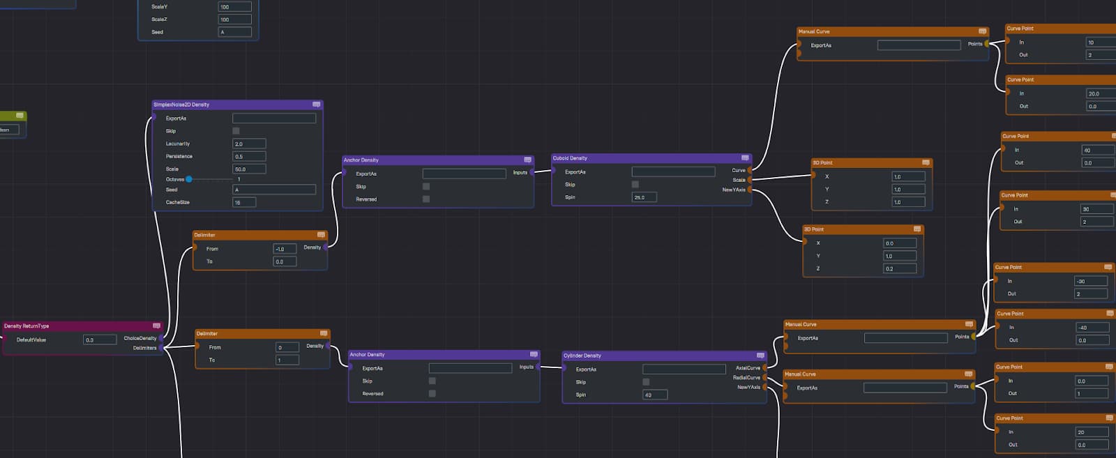
Density
The cell is populated with a Density field. The Density field is picked from a list of Delimiters. The Delimiters are picked if the ChoiceDensity field is within their range. The ChoiceDensity field’s value is sampled at the origin position of the cell.
Below is a screenshot showing a simple example of how you can anchor any Density field you design to the origin of the cell using the Anchor Density node. Below the screenshot you can see the configuration I used for that.
Parameters:
| Name | Description |
|---|---|
| ChoiceDensity | Density asset slot. <em>Benefits from a Cache Density.</em> Picks the delimiter to use for a Cell. This field is sampled at each Cell's origin. |
| Delimiters | list of delimiters. Assign Density fields to cells based on the ChoiceDensity value at the Cell's origin. |
| DefaultValue | decimal number. This value is used outside of cells. This can happen when the field’s MaxDistance value is smaller than the distance between some Positions. |
Curve
The Curve ReturnType allows you to use a Curve asset to define the value of the Density field in terms of its distance from the Positions.
Parameters:
| Name | Description |
|---|---|
| Curve | Curve asset slot. The Density value of each cell is defined by the curve. The curve’s input is the distance in blocks between the closest Position, and the Curve’s output becomes the field’s value. |
Distance
The Distance ReturnType works like the traditional CellNoise’s “Distance” return type.
It has no parameters.
Distance2
The Distance2 ReturnType works like the traditional CellNoise’s “Distance2” return type.
It has no parameters.
Distance2Add
The Distance2Add ReturnType works like the traditional CellNoise's "Distance2Add" return type.
It has no parameters.
Distance2Sub
The Distance2Sub ReturnType works like the traditional CellNoise's "Distance2Sub" return type.
It has no parameters.
Distance2Mul
The Distance2Mul ReturnType works like the traditional CellNoise's "Distance2Mul" return type.
It has no parameters.
Distance2Div
The Distance2Div ReturnType works like the traditional CellNoise's "Distance2Div" return type.
It has no parameters.
DistanceFunction
Determines the way in which the distance to the closest Position is calculated. Currently there are two types: Euclidean and Manhattan.
No Parameters.
Distance
The Distance outputs a value in function of the distance from the origin 0 of the field. The provided Curve asset maps the distance to the output Density value.
Expected Inputs: 0
Parameters:
| Name | Description |
|---|---|
| Curve | Curve asset slot. Maps the Distance from the origin to a Density value. |
Ellipsoid
The Ellipsoid is a deformed Sphere. You can use a Scale vector to stretch and compress the Sphere in different directions. You can spin it by giving it a new Y axis and a spin angle (in degrees).
The order of deformations done to the Sphere is as follows:
- Stretch and compress using the Scale vector.
- Align its Y axis to the provided one.
- Spin it around the new Y axis.
Below is an example Ellipsoid and its assets.
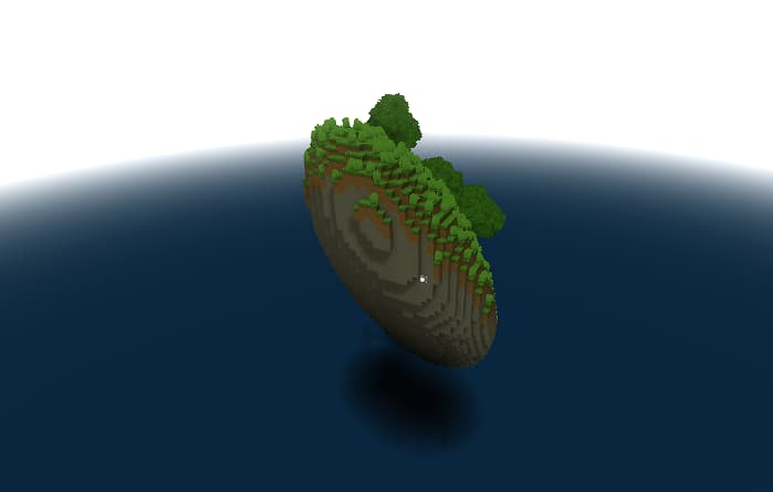
Expected Inputs: 0
Parameters:
| Name | Description |
|---|---|
| Curve | Curve asset slot. Maps the Distance from the origin to a Density value. |
| Scale | 3D vector asset slot. Determines how much to stretch the Sphere in each direction. |
| NewYAxis | 3D vector asset slot. Let’s you rotate the field around its origin. |
| Spin | decimal number. Determines the angle in degrees by which to spin the Ellipsoid around its Y axis. |
Cube
The Cube outputs a Density value in function of the distance from the origin axis of the field. The provided Curve asset maps the distance to the output Density value.
Expected Inputs: 0
Parameters:
| Name | Description |
|---|---|
| Curve | Curve asset slot. Maps the Distance from the origin to a Density value. |
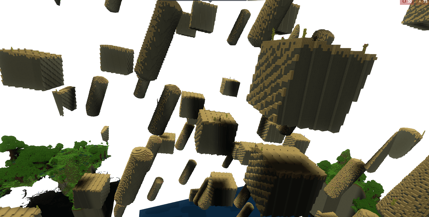
Cuboid
The Cuboid is a deformed Cube. You can use a Scale vector to stretch and compress the Cube in different directions. You can spin it by giving it a new Y axis and a spin angle (in degrees).
The order of deformations done to the Cube is as follows:
- Stretch and compress using the Scale vector.
- Align its Y axis to the provided one.
- Spin it around the new Y axis.
Below is an example cuboid and its assets.
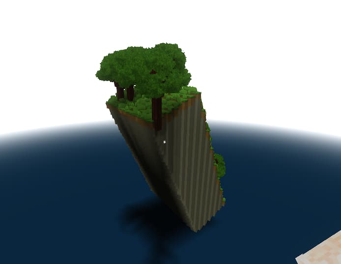
Expected Inputs: 0
Parameters:
| Name | Description |
|---|---|
| Curve | Curve asset slot. Maps the Distance from the origin to a Density value. |
| Scale | 3D vector asset slot. Determines how much to stretch the Cube in each direction. |
| Spin | decimal number. Determines the angle in degrees by which to spin the Ellipsoid around its Y axis. |
| NewYAxis | Point3D asset slot. Let’s you rotate the field around its origin. |
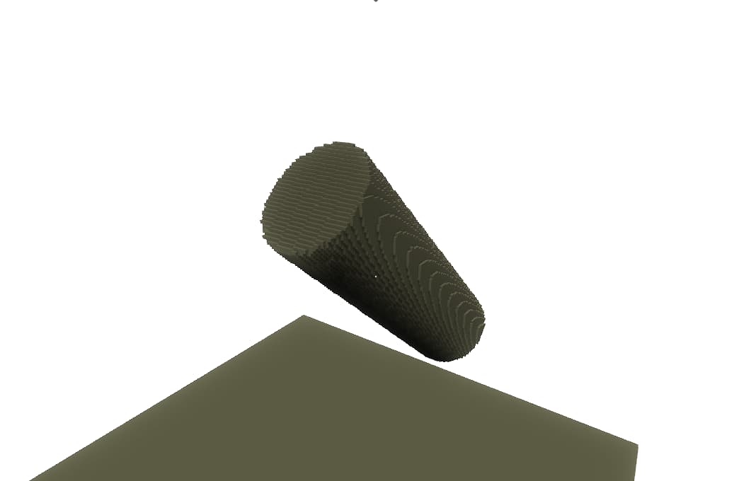
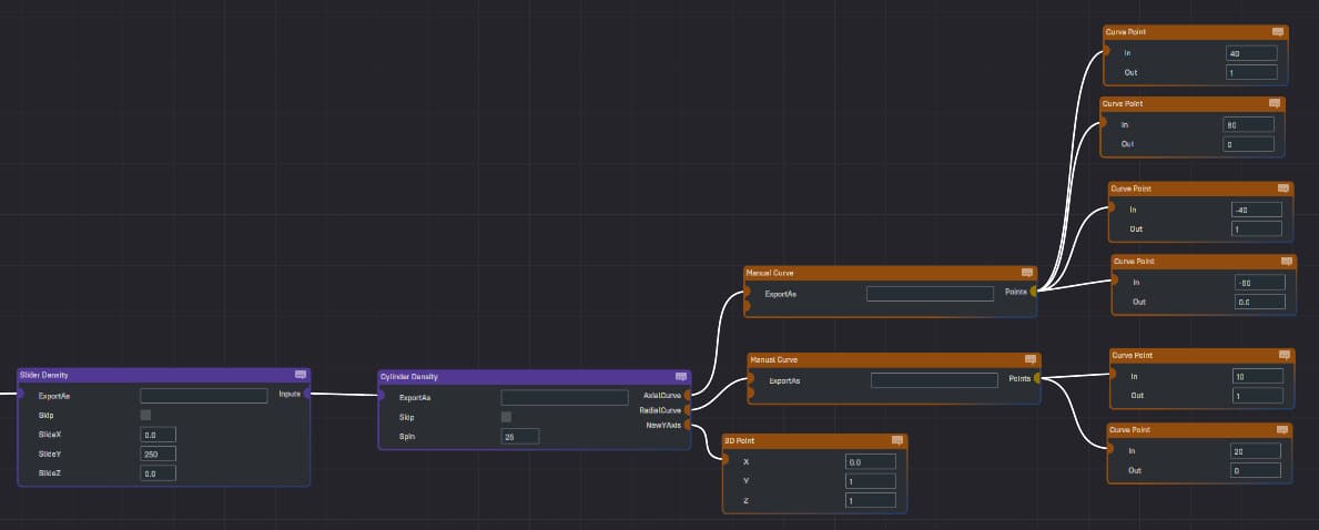
Cylinder
The Cylinder generates a cylindrical shape, crazy I know. You can spin it by giving it a new Y axis and a spin angle (in degrees).
The AxialCurve determines the Density value along its Y axis (not the world’s Y axis). The AxialCurve takes positive inputs anywhere above the Cylinder’s XZ-plane and it takes negative values anywhere below it.
The RadialCurve determines the Density value in function of the distance from the Y axis. This basically can determine how thick the Cylinder is.
Below is an example cuboid and its assets.
Expected Inputs: 0
Parameters:
| Name | Description |
|---|---|
| AxialCurve | Curve asset slot. Maps the Distance from the Cylinder’s XZ-plane to a Density value. |
| RadialCurve | Curve asset slot. Maps the Distance from the Cylinder’s Y axis to a Density value. |
| Spin | decimal number. Determines the angle in degrees by which to spin the Ellipsoid around its original Y axis. |
| NewYAxis | Point3D asset slot. In combination with the spin, this lets you rotate the Cylinder around its origin by aligning its original Y-axis with the provided one. |
Axis
The Axis outputs a Density value in function of the distance from a provided Axis line that passes through the origin 0 of the field or through the anchor point if the IsAnchored flag is true. The provided Curve asset maps the distance to the output Density value.
Expected Inputs: 0
Parameters:
| Name | Description |
|---|---|
| Axis | 3D vector asset slot. Determines the axis from which the distance is used. |
| Curve | curve asset slot. Determines the Density value at any distance from the axis. |
| IsAnchored | boolean. If true, the Axis node will anchor itself to the closest anchor. Although you could use an Anchor node to anchor an Axis Density node, this internal method doesn’t produce some artifacts. |
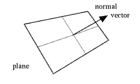
Plane
The Plane Density node allows you to define a Density field in function of the distance from a user-defined plane that passes through the field’s origin 0 or through the anchor if the flag IsAnchored is enabled. You can granularly define the Density value using a Curve asset. The PlaneNormal vector determines the direction the plane is facing.
Expected Inputs: 0
Parameters:
| Name | Description |
|---|---|
| PlaneNormal | 3D vector asset slot. Determines the direction the plane is facing. |
| Curve | curve asset slot. Determines the Density value at any distance from the plane. |
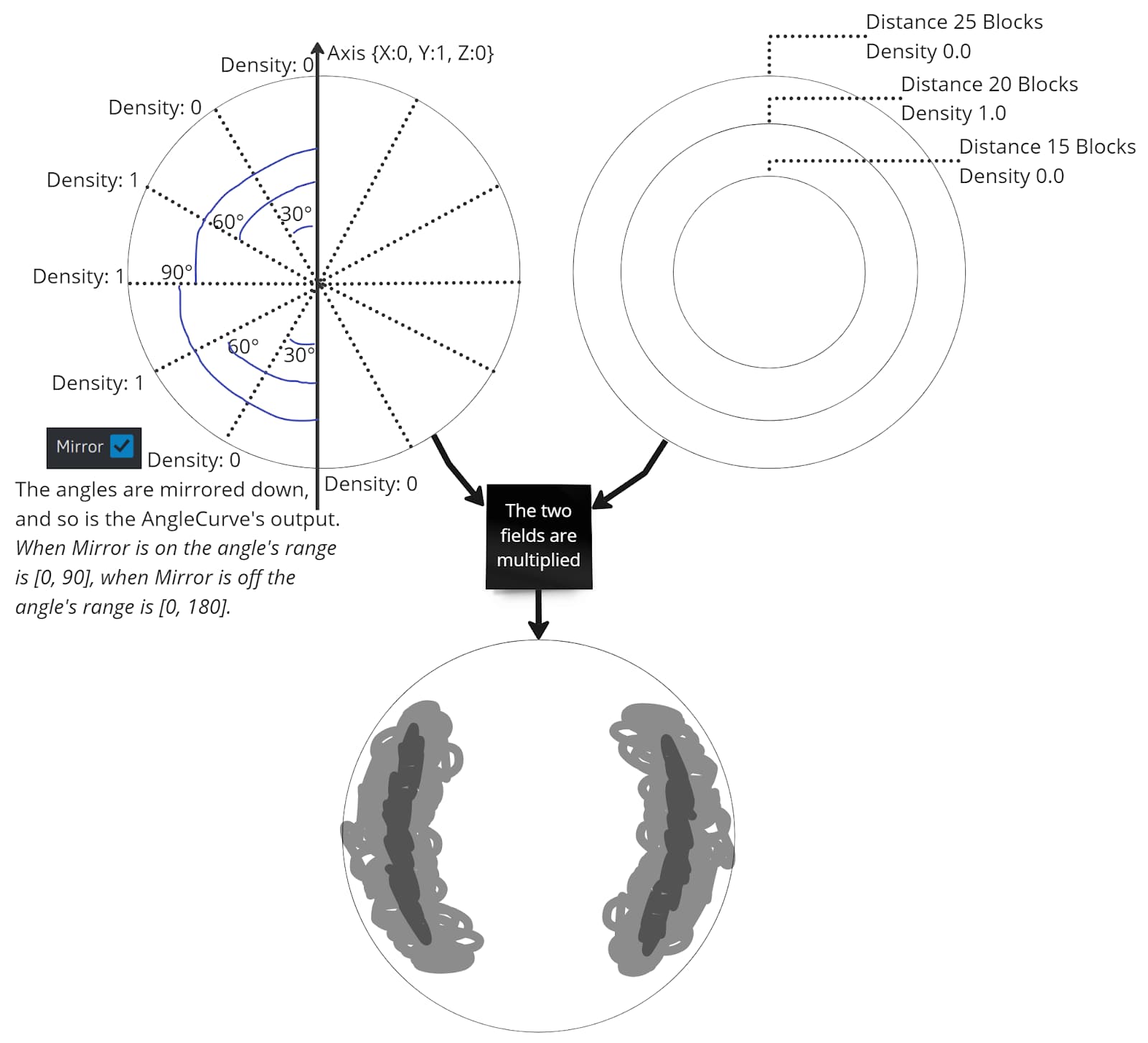
Shell
The Shell Density node allows you to define regions of the shell around the origin 0 of the field based on the direction and the distance from origin. The angles, thickness and Density values of the shell are fully configurable through Curve assets.
The diagram below shows the anatomy of the Shell node and how its AngleCurve and its DistanceCurve are multiplied to obtain the result in the screenshot.
Expected Inputs: 0
Parameters:
| Name | Description |
|---|---|
| Axis | 3D vector asset slot. Determines the axis against which the angle is calculated. |
| Mirror | boolean value. If true then the angle is mirrored in both directions of the axis. |
| AngleCurve | curve asset slot. Determines the Density value at any given angle from the axis. |
| DistanceCurve | curve asset slot. Determines the Density value at any distance from the origin. |
CurveMapper
This node maps the input to a Curve.
Expected Inputs:
- 0: Density to remap.
Parameters:
| Name | Description |
|---|---|
| Curve | curve. Maps the input Density value. |
Mix
Mixes two inputs. How much of each input to use in the mix is gauged by a third input called the gauge:
- Where the Gauge is less or equal to 0.0: only Density A is used.
- Where the Gauge is more or equal to 1.0: only Density B is used.
- Where the Gauge is between 0.0 and 1.0: Density A and B are mixed proportional to the Gauge.
Expected Inputs: 3
- 0: Density A.
- 1: Density B.
- 2: Gauge.
Parameters: None
MultiMix
Mixes multiple inputs. How much of each input to use in the mix is gauged by the last input called the Gauge.
The inputs are ordered top-down (in the node editor) and each input is assigned an index: starting with 0 for the top one and incrementing downwards.
The keys let you pin the different inputs to Gauge values. Where the Gauge input's value approaches a Key's value, the input referenced by that Key is stronger in the final result.
Expected Inputs: unlimimied, the last one is the Gauge.
Parameters: None
Sum
The output is the sum of all the inputs.
Expected Inputs: [0, infinite)
This node has no parameters.
Multiplier
The output is the multiplication of all the inputs.
The Multiplier node skips the remaining inputs after an input provides a Density value of 0. This can help you optimize your Density performance by ordering the Multiplier inputs with the cheapest mask first.
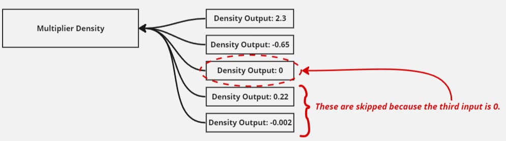
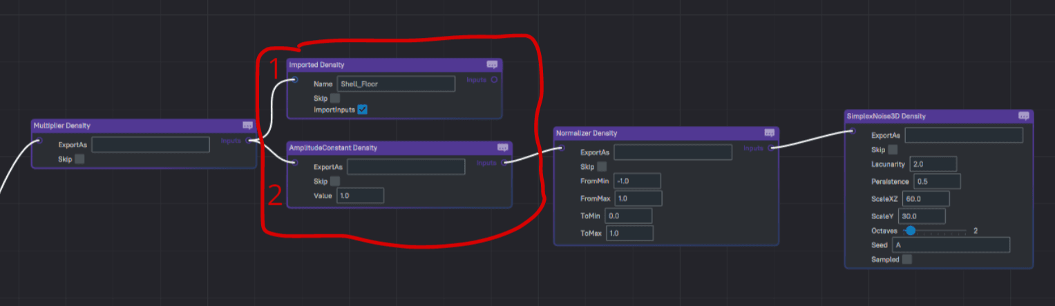
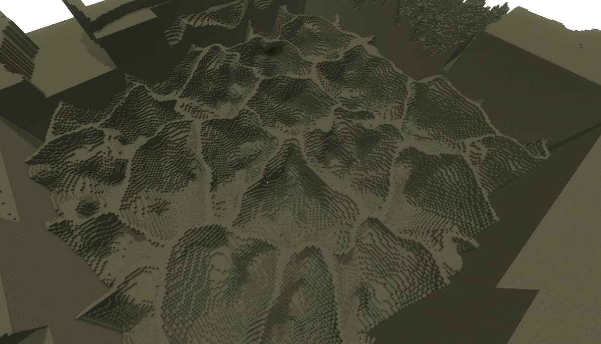
The image below is an example where I put the edge's shell first in the Multiplier's input list, and the noise second. I configured the shell to be 0 where I want to mask it out. As a result, the noise (more expensive than the shell) is not calculated for large volumes of space where the shell mask is 0, and I got a performance improvement of ~40%. This is because around that percentage of the volume in that setup was masked out by the shell.
Expected Inputs: [0, infinite)
This node has no parameters.
Max
The output is the greatest value of all the inputs. If no inputs are provided it is 0.
Expected Inputs: [0, infinite)
This node has no parameters.
Min
The output is the smallest value of all the inputs. If no inputs are provided it is 0.
Expected Inputs: [0, infinite)
This node has no parameters.
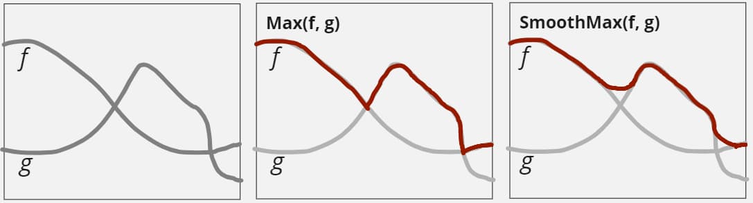
SmoothMax
The output is a smoothed maximum between the two inputs. The diagram below compares a smooth maximum and a normal maximum of functions f and g. The normal maximum has sharp angles where f and g cross.
Expected Inputs: 2
Parameters:
| Name | Description |
|---|---|
| Range | positive decimal number. Greater values result in more smoothing. A good starter value could be 0.2. |
SmoothMin
The output is a smoothed minimum between the two inputs. This node works the same as SmoothMax, please read that node’s description.
Expected Inputs: 2
Parameters:
| Name | Description |
|---|---|
| Range | positive decimal number. Greater values result in more smoothing. A good starter value could be 0.2. |
Clamp
This node ensures that the output is within the provided range which is defined by the two wall parameters. Input values that are inside the range don’t change and inputs values outside the range are brought back to the range’s extreme.
Expected Inputs: 1
Parameters:
| Name | Description |
|---|---|
| WallA | any decimal number |
| WallB | any decimal number |
SmoothClamp
This node ensures that the output is within the provided range which is defined by the two wall parameters. The concept is similar to the Clamp node documented above, but the output is smoothed to the limits by the provided range value.
Expected Inputs: 1
Parameters:
| Name | Description |
|---|---|
| WallA | any decimal number |
| WallB | any decimal number |
| Range | decimal values above 0. Larger values result in smoother transition when the input approaches or exceeds the walls. |
Abs
The output is the absolute value of the input.
Expected Inputs: 1
This node has no parameters.
XValue
The local X coordinate.
Expected Inputs: 0
Parameters: None
YValue
The local Y coordinate.
Expected Inputs: 0
Parameters: None
ZValue
The local Z coordinate.
Expected Inputs: 0
Parameters: None
XOverride
Overrides the X coordinate the input sees.
Expected Inputs: 1
Parameters: None
YOverride
Overrides the Y coordinate the input sees.
Expected Inputs: 1
Parameters: None
ZOverride
Overrides the Z coordinate the input sees.
Expected Inputs: 1
Parameters: None
YSampled
Reduces the performance cost of its child Density by interpolating between spread-out samples along the Y-axis.
Instead of generating the child's Density value for every single coordinate, it generates the child's value in intervals determined by the SampleDistance and SampleOffset and interpolates the value between the samples.
Tips:
- Upstream transformations and warping of the domain could drastically reduce any performance gains.
- If the downstream Density doesn't cost more to generate vertically then this node won't have a significant impact.
- 3D noise in the downstream will be sped up.
- 2D noise in the downstream will not be significantly sped up if at all.
- Use the SampleOffset to reduce undesired effects such as alignment of the interpolation artifacts with fluid levels.
- You can use this in combination with a Mix to transition to the full non-sampled version of the child node in areas where precision is important (close to a POI, at the terrain's surface, etc.).
Below you can see the performance difference between different SampleDistance values for the terrain configuration in the screenshot below:
| SampleDistance | TerrainStage (ms) |
|---|---|
| None | 14 |
| 4 | 8 |
| 8 | 6 |
| 16 | 5 |
Expected Inputs: 1
Parameters:
| Name | Description |
|---|---|
| SampleDistance | positive decimal number. Safe starting value: 4.0. Determines how far apart the samples are taken. Larger numbers result in more performance savings but less precise terrain vertically. |
| SampleOffset | decimal number. Safe starting value: 0.0. Allows for non-zero-aligned sample distribution. |
| Interpolate | boolean. Enables the smooth interpolation between the samples. |
Cache
Caches the input for the current coordinates. The capacity determines how many coordinates' can be cached before having to drop the oldest one.
Expected Inputs: 1
Parameters:
| Name | Description |
|---|---|
| Capacity | positive Integer. Determines how many coordinates this cache can hold at once. A safe value is 3. |
Angle
The angle in degrees between two vectors, one of which is procedurally generated by a VectorProvider.
Expected Inputs: 0
Parameters:
| Name | Description |
|---|---|
| Vector | 3D vector. Reference vector to compare against. |
| VectorProvider | procedural vector. Vector to compare. |
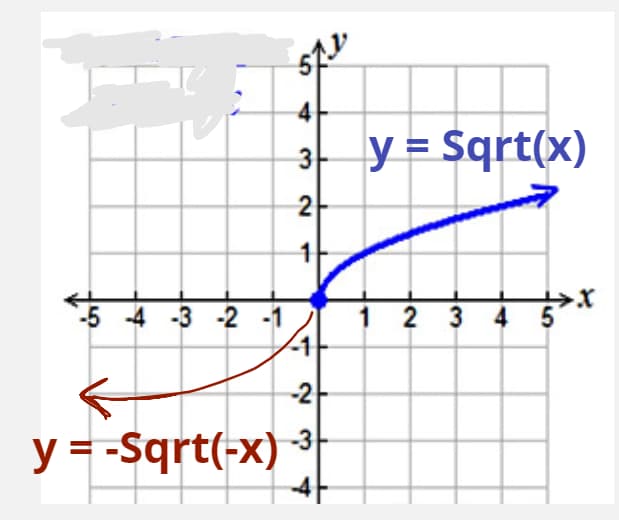
Sqrt
The output is the square root value of the input.
For negative inputs, this node uses a modified function to always return values that make sense and are useful. The following graph shows in blue the values for positive inputs, and in red the values for negative inputs.
Expected Inputs: 1
This node has no parameters.
Inverter
The output is the input multiplied by -1.
Expected Inputs: 1
This node has no parameters.
Pow
The output is the input taken to the power of the given exponent.
For negative inputs, this node uses a modified function to always return values that make sense and are useful.
Expected Inputs: 1
Parameters:
| Name | Description |
|---|---|
| Exponent | any value. A good starting value would be 2. |
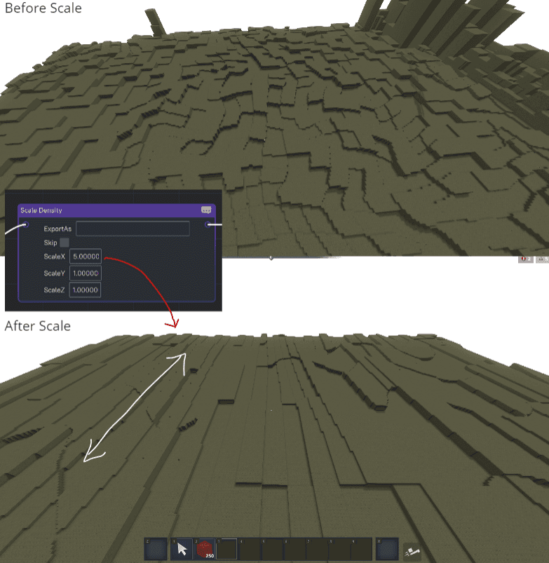
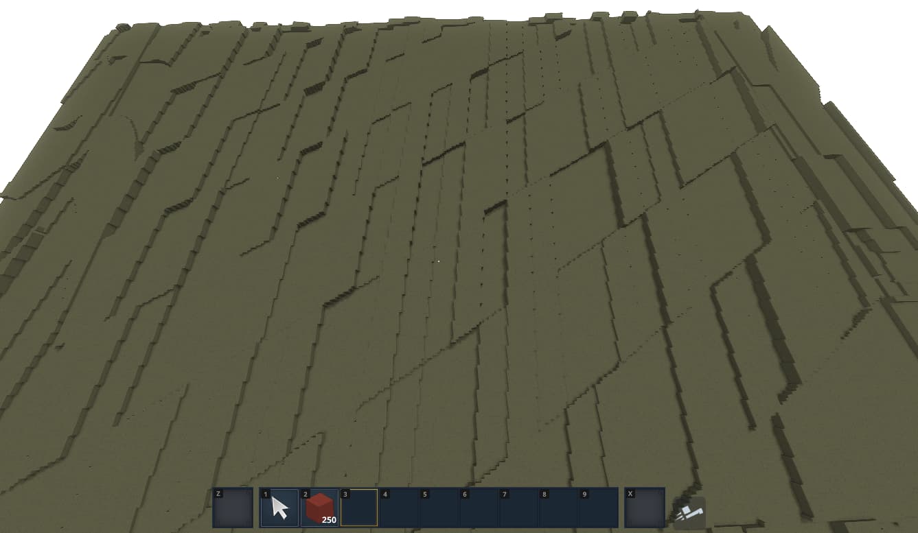
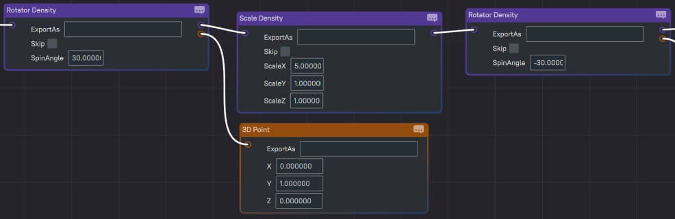
Scale
Stretches or contracts the input Density field. The input’s Density field is scaled by the factor’s provided for each axis. Values above 1 stretches the field and values below 1 contract it. Values under 0 flip the field.
The image below shows a Density field before and after passing it through a Scale node: The node is configured to only scale up the X direction.
You can also scale on a non-orthogonal axis by using Rotator nodes in combination with a Scale node, like this:
Expected Inputs: 1
Parameters:
| Name | Description |
|---|---|
| X | decimal number |
| Y | decimal number |
| Z | decimal number |
DistanceToBiomeEdge
Outputs the distance to the nearest biome edge in blocks.
Expected Inputs: 0
Parameters: None
Terrain
Outputs the world's interpolated terrain Density.
This should only be used as part of a biome's MaterialProvider nodes. This won't work if used in the Terrain's Density nodes.
Expected Inputs: 0
Parameters: None
Rotator
Aligns the input Density field so that its Y axis is aligned with the provided axis, and spins it around the new axis by the provided angle.
Expected Inputs: 1
Parameters:
| Name | Description |
|---|---|
| NewYAxis | 3D vector asset. Y-axis of the rotated field rlative to the parent's y-axis. |
| SpinAngle | decimal number. The angle in degrees to spin the field around the new axis. |
Slider
Slides the input Density field in the direction of the provided vector.
Expected Inputs: 1
Parameters:
| Name | Description |
|---|---|
| SlideX | decimal number |
| SlideY | decimal number |
| SlideZ | decimal number |
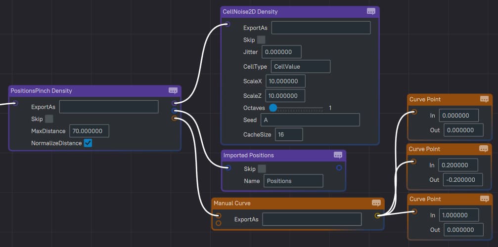
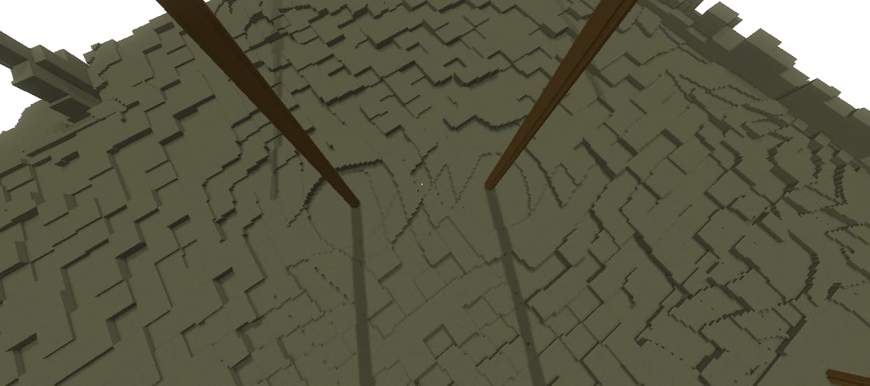
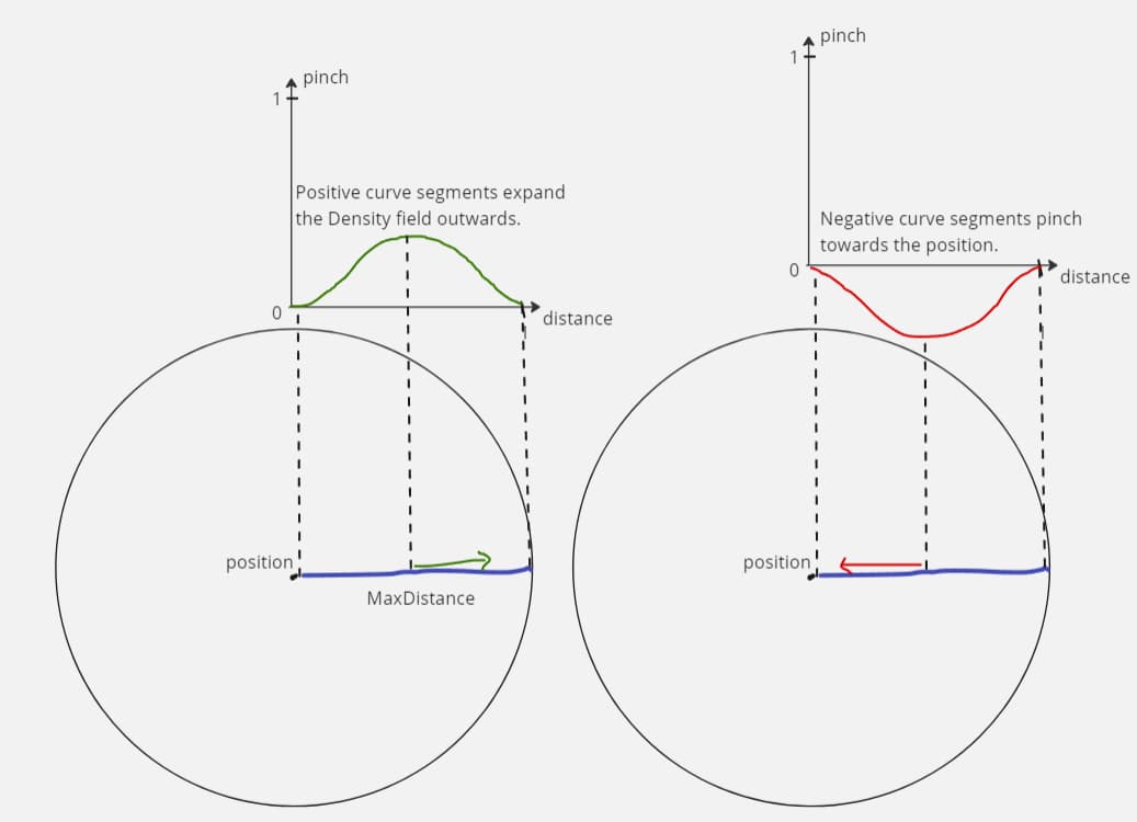
PositionsPinch
Pinches or expands the first input’s Density field around the Positions. The intensity and look of the effect is determined by the PinchCurve. The range of the effect around each position is determined by the MaxDistance.
If the NormalizeDistance is true, then the curve’s input and output’s unit is normalized to the MaxDistance. In other words, for half of the MaxDistance, the curve’s input and output will be 0.5, and at the full MaxDistance, it would be 1. Otherwise if false, the curve’s values will represent the absolute distance in terms of blocks for both its input and output.
Below is an example configuration of a pinch, and the resulting terrain.
Below is an example configuration of a pull and the resulting terrain.
The PositionsMinY and PositionsMaxY parameters limit the vertical range queried from the Positions field. The default values are 0.0 and 0.0001 to let in all the Positions at Y:0.
Expected Inputs: 1
Parameters:
| Name | Description |
|---|---|
| Positions | Positions asset slot. The Positions are the anchors that pinch and expand the Density field around them. |
| PinchCurve | Curve asset slot. The curve determines how the Density field is pinched or expanded depending on how close it is to a position. |
| MaxDistance | positive decimal number. The value represents how big the area of effect is in block units. |
| NormalizeDistance | boolean value. Default is true. If true then the Curve’s input and output unit is normalized to the MaxDistance value, otherwise if false the Curve’s input and output unit is in blocks. |
| HorizontalPinch | boolean value. Default is false. If true, the input is pinched horizontally only. |
| PositionsMaxY | decimal number. Determines the upper Y level bound of the region queried from the Positions field. Any Positions that are at or above this value are ignored. |
| PositionsMinY | decimal number. Determines the lower Y level bound of the region queried from the Positions field. Any Positions that are below this value are ignored. |
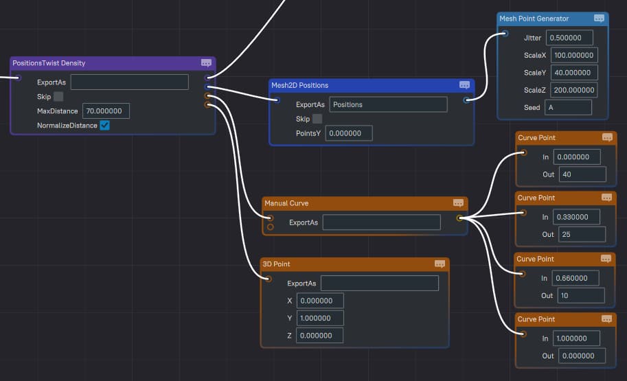
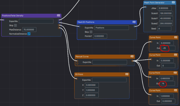
PositionsTwist
Twists the first input’s Density field around the Positions. The intensity and look of the effect is determined by the TwistCurve. The range of the effect around each position is determined by the MaxDistance.
If the NormalizeDistance is true, then the curve’s input unit is normalized to the MaxDistance. In other words, for half of the MaxDistance, the curve’s input will be 0.5, and at the full MaxDistance, it would be 1. Otherwise if false, the curve’s values will represent the absolute distance in terms of blocks.
The output of the curve is always in degrees. This means that to produce a full twist around the axis, the curve must output 360 (degrees).
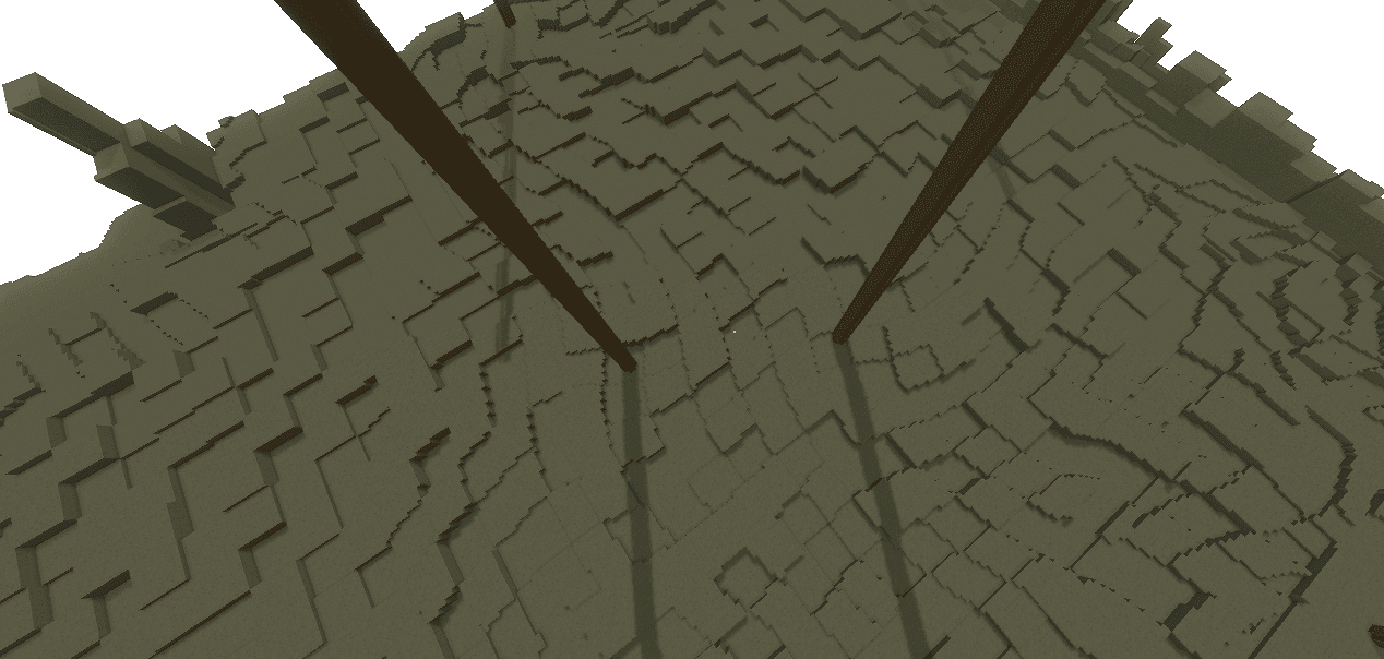
Below is an example configuration of a simple twist, and the resulting terrain.
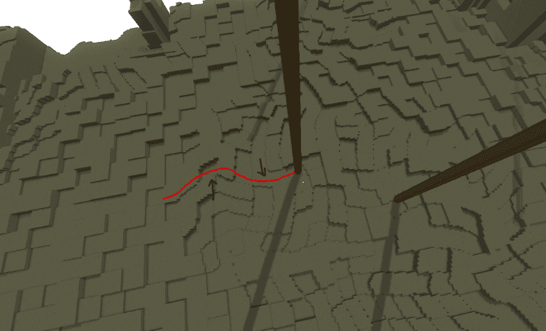
Below is an example configuration of a double twist where part of the curve twists in one direction and part in the other direction, and the resulting terrain.
Expected Inputs: 1
Parameters:
| Name | Description |
|---|---|
| Positions | Positions asset slot. The Positions are the anchors that pinch and expand the Density field around them. |
| TwistCurve | Curve asset slot. The curve determines how the Density field is twisted depending on how close it is to a position. |
| TwistAxis | vector asset slot. The axis around which the twisting happens. |
| MaxDistance | positive decimal number. The value represents how big the area of effect is in block units. |
| NormalizeDistance | boolean value. Default is true. If true then the Curve’s input unit is normalized to the MaxDistance value, otherwise if false the Curve’s input unit is in blocks. |
| ZeroPositionsY | boolean value. Flattens the positions input to y=0. |
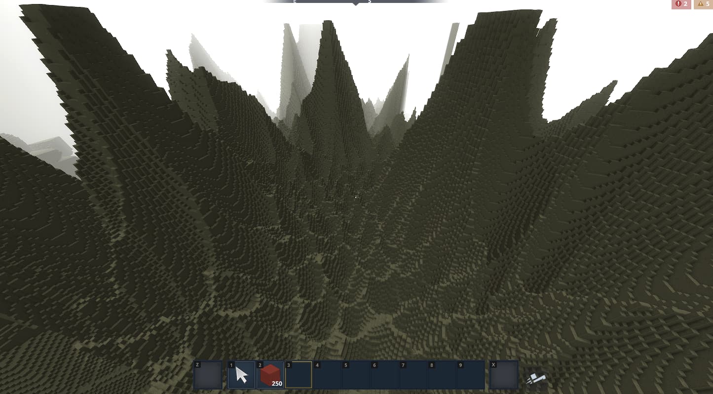
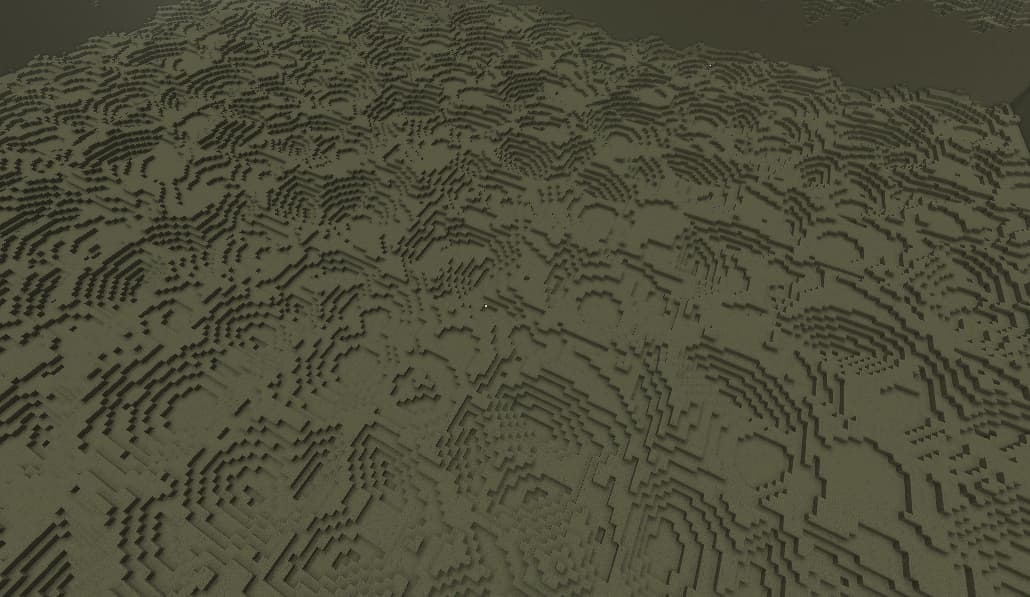
GradientWarp
Warps the first input based on the gradient of the second input Density field. This works similar to the legacy warping functionality, except it also works in 3D and you can plug any Density field into it.
This implementation is relatively expensive because it calculates the gradient of the input Density field. I recommend optimizing the use of this node by isolating and minimizing its use space. A fast version of this node can be implemented which would let you only use Simplex noise to warp. This will depend on the feedback and priorities.
This node incorporates a Cache2D so you don’t need to use a Cache2D node on its output.
Expected Inputs: 2
- 0: Density that is warped.
- 1: Warping source.
Parameters:
| Name | Description |
|---|---|
| SampleRange | Distance between samples. Recommended value: 1. |
| WarpFactor | With greater values you get more warping. |
| 2D | If true the output of this node is 2D. An internal Cache2D is used. |
| YFor2D | Default is 0. The Y coordinate used from the input to calculate the gradient from. |
FastGradientWarp
This is a faster implementation of the GradientWarp node. It warps the input Density field using an internal simplex noise generator.
Expected Inputs: 1
- Input 1: Density field to be warped.
Parameters:
| Name | Description |
|---|---|
| WarpScale | This determines the scale of the internal warper noise field. |
| WarpLacunarity | The lacunarity of the internal simplex field. |
| WarpPersistence | The persistence of the internal simplex field. |
| WarpOctaves | The internal field’s octaves. |
| WarpFactor | The maximum distance coordinates can be warped. |
VectorWarp
Warps the input along the provided vector. The amount of warping is determined by the intensity of the second input Density field and the WarpFactor.
For example, if your warp field (second input) has a value of 0.5 and the WarpFactor is 15, then the number of blocks the first input will be warped by in the direction of the vector is 7.5 units (blocks),15 x 0.5 = 7.5.
Below is a PositionsCellNoise (Distance2Div) passed through a VectorWarp. The warping field is a normal simplex, the WarpVector is sideways 1 and the WarpFactor is 15.
Expected Inputs: 2
- Input 1: Density field to be warped.
- Input 2: Density field that warps the first field.
Parameters:
| Name | Description |
|---|---|
| WarpFactor | With greater values you get more warping. |
| WarpVector | Can be any vector. This determines the direction in which the warping happens. Negative values of the factor or the warping density field will result in flipped warping direction. |
Anchor
Anchors the origin of the child field (input) to the contextual Anchor if it exists. It basically puts the 0 origin of the child Density at the position of the Anchor.
For a contextual Anchor to exist, a parent of this node must produce an Anchor. The Density ReturnType node, for example, leaves the cell's center as a contextual Anchor in its Density child’s context.
You can also reverse the effect later down the line to move the origin back to the world’s origin like in the screenshot below. The field is unanchored when it reaches the bottom branch of the Sum, but the top branch is still anchored.
Example: Say you have a Density field that creates a ball around its origin 0. You also have a PositionsCellNoise with a Density return type, which leaves an anchor point at its cell's center. If you anchor the ball Density to the cell, the ball will generate around the cell's center.
Expected Inputs: 1
Parameters:
| Name | Description |
|---|---|
| Reverse | If true, the node will reverse the origin of the child to the world’s origin, or the origin before the previous Anchor node. |
Normalizer
It linearly remaps the input's range. The scale is defined by the FromMin, FromMax, ToMin and ToMax parameters. The diagrams below show how those four parameters can be intuitively used to normalize the input.
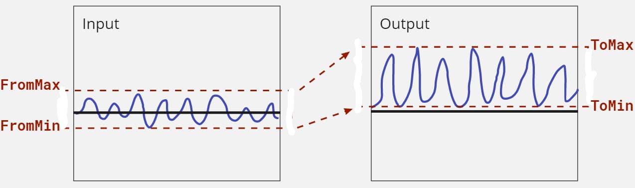
Note that the FromMin and FromMax can be any values, in this example I decided to place them at the extremes of the input’s range.
Expected Inputs: 1
Parameters:
| Name | Description |
|---|---|
| FromMin | any decimal number. The value that will be remapped to ToMin. |
| FromMax | any decimal number. The value that will be remapped to ToMax. |
| ToMin | any decimal number. The value that FromMin will be remapped to. |
| ToMax | any decimal number. The value that FromMax will be remapped to. |
BaseHeight
This node lets you reference a DecimalConstant from the WorldStructure. It can operate in 2 modes:
- Distance OFF: output the Y value of the BaseHeight at each X/Z position
- Distance ON: output the distance between the queried position and the BaseHeight.
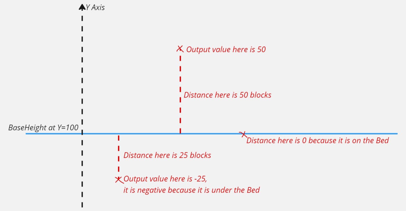
In Distance mode ON, the output is measured in blocks (coordinate units). The value is positive if the query position is above the BaseHeight, and negative if it is below the BaseHeight. Below is an example of that.
Expected Inputs: 0
Parameters:
| Name | Description |
|---|---|
| BaseHeightName | Name of the DecimalConstant to reference. |
| Distance | Toggles whether to output the raw Y coordinate of the BaseHeight or the distance from the BaseHeight from the query position. |
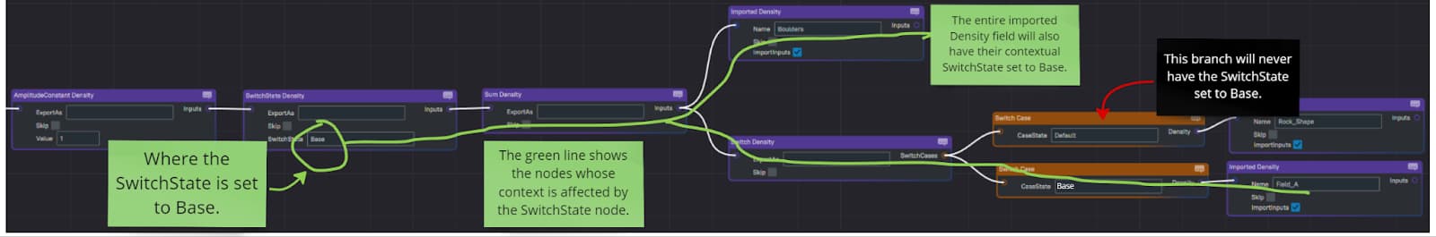
Switch
Lets you switch between multiple Density branches based on the contextual SwitchState. The SwitchState is a string that can be placed in the context of a Density tree using a SwitchState Density node. The default SwitchState of a Density tree is “Default”.
Below is an example where I use a Default branch, alongside two other branches.
Expected Inputs: 0
Parameters:
| Name | Description |
|---|---|
| SwitchCases | The possible paths to switch into based on the parent's SwitchState. |
SwitchState
Sets the contextual SwitchState for the downstream Density branch.
See the Switch documentation above for an example use case.
Expected Inputs: 1
Parameters:
| Name | Description |
|---|---|
| SwitchState | Name of the SwitchState to set for the children of this node. |
Imported
Imports an exported Density asset.
Parameters:
| Name | Description |
|---|---|
| Name | string. The exported Density to import. |
Exported
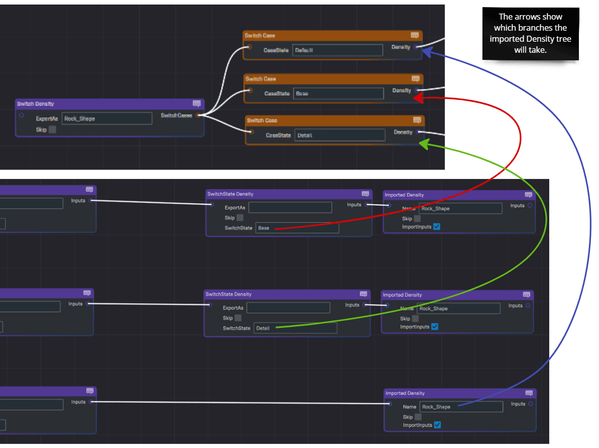
Allows exporting a Density field as a single instance. Enabling the SingleInstance on this node ensures all importers share the same logic.
By default a completely different instance is create for every Imported node. When there are multiple Imported nodes that import the same exported key, a new instance of that exported Density tree will be created for each one of the Imported nodes. SingleInstance ensures all importers share the same underlying instance of the node tree.
This node can be used to optimize caching when an exported Density is imported multiple times in the same context and contains caches. The caches would be shared between the different imported instances.
Important: This is still an experimental feature and could cause unexpected behaviors if misused.
Expected Inputs: 1
Parameters:
| Name | Description |
|---|---|
| SingleInstance | Enable to share the exported for all Imported nodes referencing this key. |